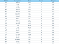
The table shows the Survey name, the International Council for the Exploration of the Sea (ICES) sub-division in which the survey is undertaken, the gear used in the survey, the initial start date of the survey and the quarter used for the assessments.

The figure shows concentrations of CB188 relative to the assessment criteria BAC (Background Assessment Concentration) and EQS (Environmental Quality Standard as given in the Water Framework Directive). For instance, a point at '4x EQS' indicates a site where the observed concentration was four (4) times the EQS limit. The points have been spread in the x direction in order to avoid too much overlap.

The figure shows the percentage of monitoring sites with threshold exceedances of pesticides in surface waters, different sized rivers, lakes and groundwater in European countries. This was used to examine threshold exceedances according to Surface Waters; Rivers, small; Rivers, medium; Rivers, large; Lakes, and Groundwater.

The figures show the percentage of monitoring sites with exceedance of effect thresholds or quality standards, set by European or national regulatory standards, and weighted by country area to reduce the impact of uneven data reporting.
For surface waters, EU environmental quality standards and (in the absence of those) national regulatory standards were used, reflecting the lowest ecotoxicologically-based effect threshold. Effect thresholds were identified for 116 out of 237 pesticides (49%). The exceedances included here refer to those 116 pesticides.
For groundwater, the Groundwater Directive quality standard of 0.1µg/l was used to identify exceedance. Twelve non-relevant metabolites (nrM) were excluded from the assessment.

The maps show trends in annual 25-percentile of oxygen concentrations in near-bottom waters at stations with at least 6 years of observations in the period 1989-2021, and the number of trends for the North-East Atlantic and Baltic Sea, by three classes of DO concentrations: <4mg/l (including <2mg/l class); 4-6mg/l and >6mg/l. Only trends for time series ending after 2000 are included.
The chart shows the number of time series with increasing trend/no trend/decreasing trend in the North-East Atlantic Ocean and Baltic Sea for grid cells with concentrations <4 mg/l, 4-6 mg/l and >6 mg/l group, for oxygen concentrations in the near-bottom layer during 1989-2021.
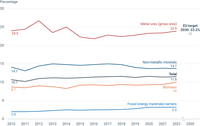
The black line indicates changes in the total circular material use rate for the EU over time, while the coloured lines show changes in the circular material use rates for the various material groups.
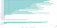
Cluster columns chart shows development in landfill rate of municipal waste in European countries in 2010 and 2021. Data is presented in descending order according to 2021 data values. Line chart represents EU landfill target for 2035.

The figure combines two charts. The stacked chart shows the amounts and percentage of waste (excluding major mineral waste) deposited in landfills in the EU-27. The line chart shows amounts landfilled for major waste categories (household and similar waste, combustion waste, sorting residues and other waste).
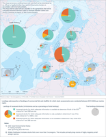
The figure shows the proportion of commercial European fish landings assessed per regional sea distinguishing between assessed and non-assessed stocks. For the assessed stocks a distinction is made between (i) landings of stocks for which information is available to determine Good Environmental Status (GES) for Fishing mortality (F) and/or Spawning Stock Biomass (SSB) and (ii) landings for stocks for which information is not available to determine GES for F and/or SSB.
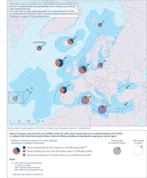
This figure shows the state of the assessed commercially exploited fish and shellfish stocks per European marine region, for which assessments were conducted in 2019-2022. Stocks for which adequate information is available to determine Good Environmental Status (GES) for fishing mortality (F) and/or reproductive capacity (spawning stock biomass (SSB)) are included (i.e. Z, total number of stocks; Y, total number of assessed stocks; and X, number of stocks for which adequate information is available to determine GES on the basis of these two criteria). A distinction is made between stocks: (1) in good status based on both fishing mortality and reproductive capacity; (2) in good status based on only one of the criteria - fishing mortality or reproductive capacity (either because one of the two criteria is not in good status or because there is only one available criteria, and it is in good status); and (3) not in good status based on both fishing mortality and reproductive capacity (may include cases where only one criteria is available and it is not in good status).

This figure shows trends in the status of assessed commercially exploited fish and shellfish stocks between 1947 and 2021, expressed in two metrics-fishing mortality (F) and reproductive capacity (i.e. spawning stock biomass (SSB))-relative to their policy thresholds for the Marine Strategy Framework Directive's 'good environmental status' (GES) (i.e. FMSY and MSY Btrigger, respectively).

The graph shows the aggregated environmental impacts associated with each of the seven consumption domains, that are caused by EU consumption, regardless of where these impacts occur.

The graph shows the level of aggregated environmental impacts associated with the consumption of each EU Member State, expressed in points per capita for the years 2010 and 2021, sorted from the country with the highest impacts to the country with the lowest impacts in 2021.
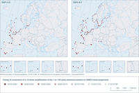
The projected probability increase of a certain extreme sea level is often presented as an amplification factor (AF) that indicates the ratio between the future and historical probability of that extreme sea level (commonly the 1-in-100 years extreme event).
The use of the historical probability of the 1-in-100 years extreme sea level combined with future projections of sea level rise, available from CMIP6 projections (Coupled Model Intercomparison Project phase 6), allow to provide and estimate of the year of occurrence for a 10 times amplification of the historical event (AF10) under an optimistic future scenario (Shared Socioeconomic Pathways SSP1-2.6) and a future one without significant emissions abatement (SSP5-8.5).
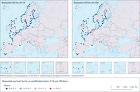
The projected probability increase of a certain extreme sea level is often presented as an amplification factor (AF) that indicates the ratio between the future and historical probability of that extreme sea level (Hermans et al., 2023).
The use of these estimates allow one to evaluate the changes of the 1-in-100 years extreme events according to sea level rise projections and provide an estimate of the requested SLR increase to determine a more frequent occurrence, e.g. 1-in-10 year (AF10) or every year (AF100).

The arrows show the observed trend in sea level relative to land since 1970 for those tide gauges along the Europe coastline with sufficiently long time series (mm/year). Projections: European sea level change for 2081–2100 for SSP5-8.5 in metres. Results use CMIP6 model projections for long term scenario (2081-2100), for SSP5-8.5, and with respect to a baseline of 1995-2014.

The left chart depicts the rise in global mean sea level from 1900 to 2022 based on two data sources. All values are relative to the average level of the period 1993-2010, during which the two datasets overlap.
The grey line (Palmer et al., 2021) shows the ensemble sea-level reconstruction (using five members) of sea level anomalies during 1900-2010 (Palmer et al., 2021; https://iopscience.iop.org/article/10.1088/1748-9326/abdaec#erlabdaecs2).
The dark grey line (CMEMS) shows the altimeter measurements corrected from the Topex-A drift at the beginning of the time series (Legeais et al., 2020), corrected for the GIA using the ICE5G-VM2 GIA model (Peltier, 2004), for the time series from 1993 to 2022.
The right chart shows global mean sea level projections under different Shared Socioeconomic Pathways (SSP) scenarios. Sea level projections considering only processes for which projections can be made with at least medium confidence are provided, relative to the period 1995-2014, for five SSP. The scenarios are described in sections TS1.3 and 1.6 and Cross-Chapter Box 1.4 of the Working Group 1 contribution. Sea level projections considering only processes for which projections can be made with at least medium confidence are provided, relative to the period 1995-2014, for five SSP. The scenarios are described in sections TS1.3 and 1.6 and Cross-Chapter Box 1.4 of the Working Group 1 contribution.